Sample Size and Power Calculations
This resource covers essential concepts of statistical power and sample size for randomized evaluations, including hands-on applications using Stata.

- Statistical power determines the ability to detect true effects in research studies.
- Sample size directly affects the precision and reliability of estimates.
- Key design decisions - effect size, variance, clustering, and compliance- all interact to determine whether a study is adequately powered.
What Is Statistical Power?
Statistical power is the probability that a study detects a true effect when one exists. A study with low power risks a Type II error: failing to detect an effect that is real. The conventional minimum threshold is 80% power, meaning a study should correctly identify the target effect at least 80% of the time.
Power matters for three interconnected reasons. Underpowered studies produce inconclusive results even when a program works, wasting resources and potentially leading to poor policy decisions. Well-powered studies justify the ethical cost of exposing participants to an intervention or control condition, since the evidence produced must be reliable enough to be worth it. Power calculations performed before data collection also force researchers to state their assumptions clearly: expected effect size, outcome variance, and study design.
For a practical step-by-step guide to running power calculations, see Guide to Power Calculations.
IPA Example: Balsakhi Tutoring Program, India
Balsakhi Tutoring Program, India (Banerjee et al., 2007)
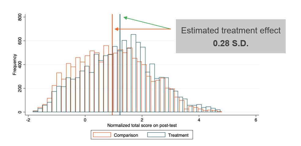
A randomized controlled trial (RCT) of the Balsakhi tutoring program enrolled 23,000 students in India. The program provided two hours of daily remedial instruction in small groups to children age 7 to 12. Test scores improved by 0.28 standard deviations (SDs) for students who received tutoring. The large sample gave the study sufficient power to detect this modest effect with confidence. If the sample had been smaller, the study might have found no statistically significant impact, not because the program failed, but because the study lacked the sensitivity to measure it.
How Sample Size Determines Precision
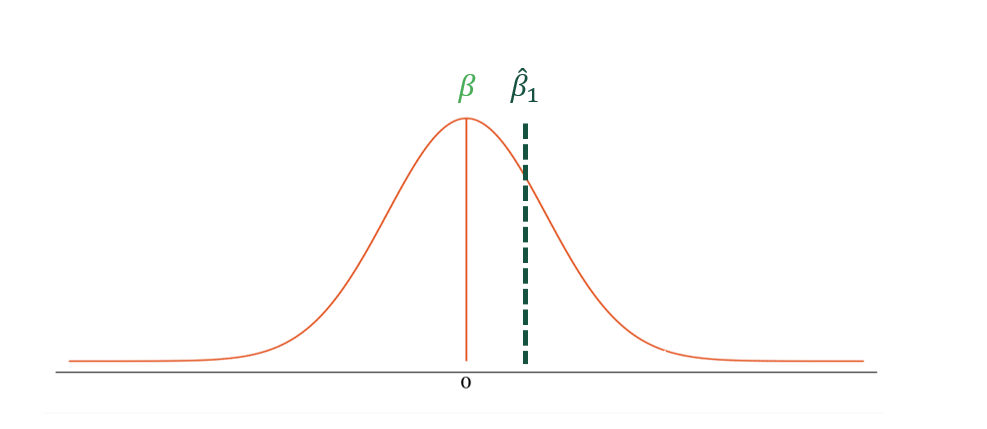
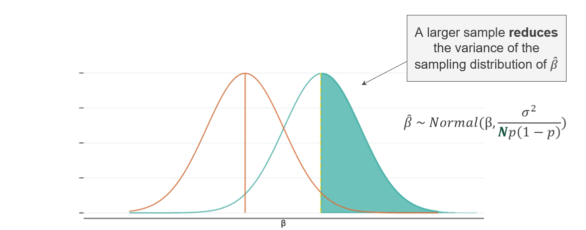
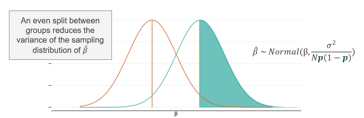
Sample size directly controls the width of the sampling distribution around any estimated treatment effect (\(\hat{\beta}\)). As \(N\) increases, estimates cluster more tightly around the true effect, reducing the risk of both false positives and false negatives. The estimated treatment effect follows a normal distribution:
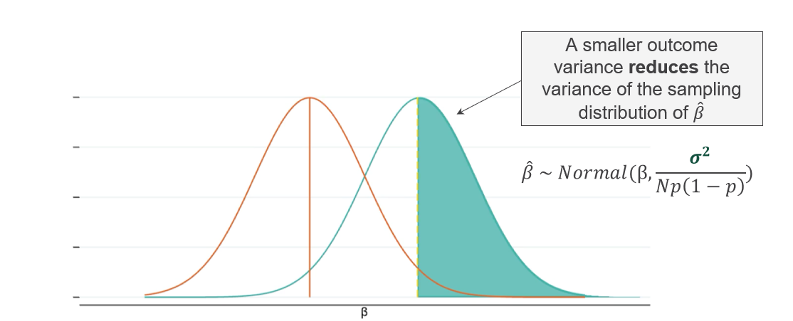
\[ \hat{\beta} \sim \mathcal{N}\left( \beta,\; \frac{\sigma^2}{N p(1 - p)} \right) \]
where \(\beta\) is the true effect, \(\sigma^2\) is the outcome variance, \(N\) is the total sample size, and \(p\) is the proportion assigned to treatment. Power increases when \(N\) grows, \(\sigma^2\) shrinks, or \(p\) approaches 0.5.
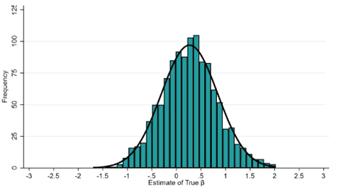
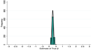
Larger samples improve power, but each additional observation has a cost in time, money, and personnel. The goal is to find the smallest sample that reliably detects an effect worth detecting.
| Factor | Effect on required sample size |
|---|---|
| Smaller expected effect size | Larger sample needed |
| Higher outcome variance | Larger sample needed |
| Lower significance level (\(\alpha\)) | Larger sample needed |
| Higher desired power (\(1 - \kappa\)) | Larger sample needed |
| Clustered or stratified design | Larger sample needed |
Statistical Inference: Errors and Thresholds
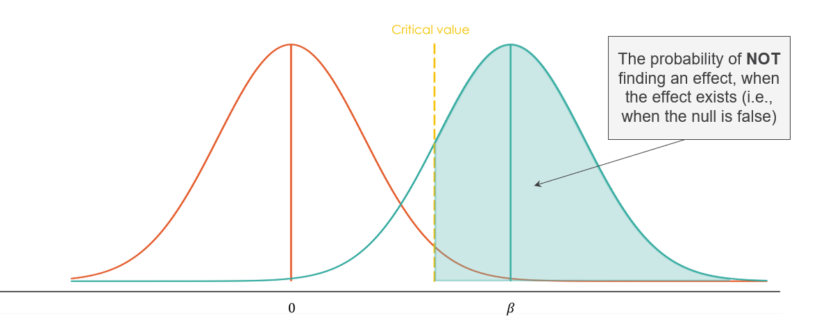
Every hypothesis test produces two possible errors. A Type I error (\(\alpha\)) occurs when a study concludes an effect exists when none does: a false positive. A Type II error (\(\kappa\)) occurs when a study misses a real effect: a false negative. Power is defined as \(1 - \kappa\).
Reducing \(\alpha\) tightens the rejection threshold, which increases \(\kappa\) and reduces power. Researchers must choose a significance level that balances these risks. The standard choice is \(\alpha = 0.05\), though values between 0.01 and 0.10 appear in the literature.
The Hypothesis Testing Framework
Step 1: State hypotheses. The null hypothesis (\(H_0\)) assumes no effect (\(\beta = 0\)). The alternative hypothesis (\(H_1\)) proposes an effect exists (\(\beta \neq 0\), or directional if one-sided).
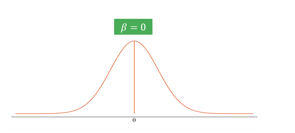
Step 2: Estimate the treatment effect. Calculate \(\hat{\beta}\) from the data and place it on the sampling distribution.
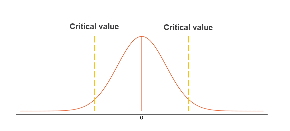
Step 3: Set critical values. At \(\alpha = 0.05\) (two-sided), the rejection regions begin at approximately ±1.96 standard errors from zero.
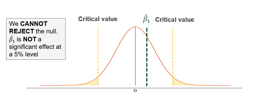
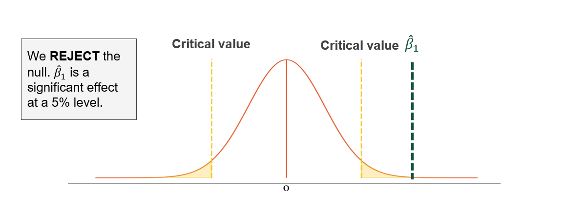
Step 4: Make a decision. If \(\hat{\beta}\) falls in the rejection region, reject \(H_0\) and conclude the effect is statistically significant. If \(\hat{\beta}\) falls within the bounds, fail to reject \(H_0\).
Power equals the proportion of the alternative distribution (\(H_1\)) that falls beyond the critical value. The less the two distributions overlap, the higher the power.
| Scenario | Underpowered study (<80%) | Well-powered study (≥80%) |
|---|---|---|
| Detection ability | True effects may be missed | True effects are likely found |
| Conclusions | Inconclusive or misleading | Clear and reliable |
| Resource use | May require repeating the study | Leads to actionable findings |
Determinants of Power
Six factors directly determine the statistical power of a study. The first four are set as visible definitions because researchers encounter them in every power calculation. Clustering and non-compliance are expanded below because they require additional context specific to field evaluations.
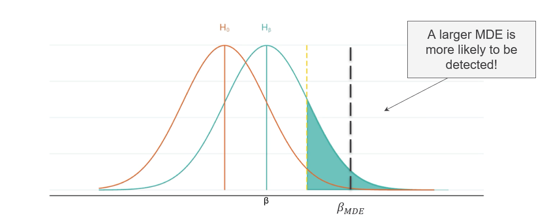
Minimum detectable effect (MDE). The MDE is the smallest treatment effect the study is designed to detect. Researchers should set it based on the smallest effect that would be policy-relevant or cost-effective to implement, not on convenience. Smaller MDEs require larger samples to achieve the same power.
Sample size (\(N\)). More observations narrow the sampling distribution and increase the probability of detecting the true effect. This is the most direct lever researchers control.
Outcome variance (\(\sigma^2\)). Higher variance in the outcome measure makes it harder to isolate the treatment signal. The most effective way to reduce residual variance is to collect a baseline measurement of the primary outcome variable. Controlling for additional covariates beyond the baseline offers only marginal gains and should not substitute for adequate sample size.
Sample allocation. Power is maximized when treatment and control groups are equal in size (\(p = 0.5\)). Unequal splits reduce power even when total \(N\) is held constant.
Many field evaluations randomize at the group level -schools, communities, or health facilities- rather than at the individual level. Individuals within the same cluster tend to be more similar to each other than to individuals in other clusters. This similarity reduces the effective information each additional observation provides and must be accounted for in power calculations.
The degree of within-cluster similarity is captured by the intra-cluster correlation coefficient (ICC), denoted \(\rho\). The design effect (DEFF) quantifies the cost of the clustered design relative to simple random assignment:
\[ DEFF = 1 + (m - 1)\rho \]
where \(m\) is the average cluster size. The required sample size under a clustered design equals the simple-random-sample size multiplied by DEFF. Typical ICC values in development economics evaluations range from 0.05 to 0.30. When ICC is high, adding more clusters increases power more efficiently than adding more individuals within existing clusters.
Ignoring clustering in power calculations when randomization occurs at the cluster level is one of the most common causes of underpowered studies. The unit of analysis in the power calculation must match the unit of randomization.
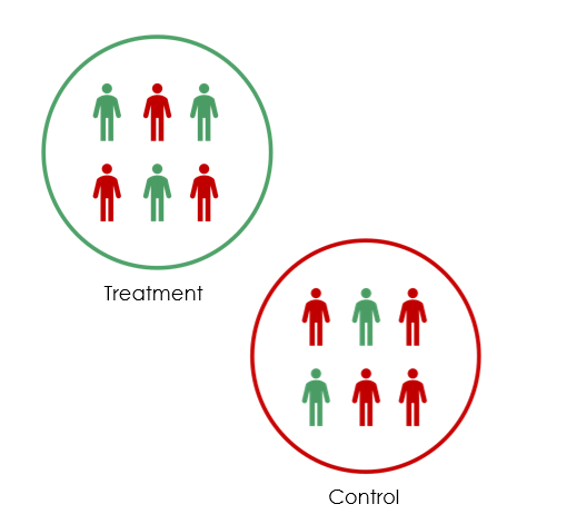
Non-compliance occurs when participants do not adhere to their assigned condition. It reduces power by compressing the estimated treatment effect toward zero, effectively shrinking the MDE. Increasing compliance is one of the strongest levers available to improve power after the study design is set.
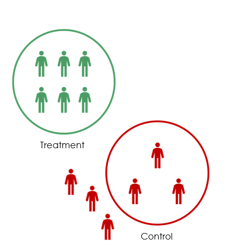
Attrition is the loss of participants during the study. It reduces power by shrinking the effective sample size. If attrition is correlated with treatment assignment -for example, more participants in the control group drop out- the estimated effect is also no longer unbiased.
Both problems are best addressed through study design: strong rapport with participants, appropriate incentives, and respondent tracking protocols established before data collection begins.
Applying Power Calculations in Stata
Stata’s power command performs sample size and power calculations and generates sensitivity tables and graphs (StataCorp 2023). The three cases below use the Balsakhi study to illustrate the main use cases.
help powerGoal: determine how many participants are needed to detect an expected effect.
Assumptions: MDE of 0.2 SD, 80% power, outcome SD of 1, individual-level randomization, perfect compliance, no attrition, no covariates.
power twomeans 0 0.2 , power(0.8) sd(1)A power of 80% requires 788 students total: 394 in the treatment group and 394 in the control group.
With a larger expected effect of 0.4 SD:
power twomeans 0 0.4 , power(0.8) sd(1)Raising the power target to 90% at 0.2 SD increases the required sample to 1,054 students:
power twomeans 0 0.2 , power(0.9) sd(1)Additional exercises: Download power.do
Goal: find the smallest effect detectable given a fixed sample size.
Assumptions: 1,000 students (500 per group), 80% power, outcome SD of 1.
power twomeans 0 , n(1000) power(0.9) sd(1)The graph below shows how the MDE shrinks as sample size increases from 500 to 1,500 students:
power twomeans 0 , n(500(250)1500) power(0.8) sd(1) graphAdditional exercises: Download power.do
Goal: determine the statistical power for a specific design.
Assumptions: 1,000 students, effect size of 0.2 SD, outcome SD of 1.
power twomeans 0 0.2 , n(1000) sd(1)Estimated power: 0.88. The graph below traces how power increases with sample size:
power twomeans 0 0.2 , n(100(100)1000) sd(1) graphAdditional exercises: Download power.do
References
Banerjee, Abhijit, Shawn Cole, Esther Duflo, and Leigh Linden. 2007. “Remedying Education: Evidence from Two Randomized Experiments in India.” Quarterly Journal of Economics 122, no. 3: 1235–1264. https://doi.org/10.1162/qjec.122.3.1235
Banerjee, Abhijit, Shawn Cole, Esther Duflo, and Leigh Linden. 2017. “Balsakhi” [dataset]. Harvard Dataverse. https://doi.org/10.7910/DVN/LIXVTF
StataCorp. 2023. Stata Power and Sample Size Reference Manual: Release 18. College Station, TX: Stata Press. https://www.stata.com/manuals/power.pdf
Additional Resources
Abdul Latif Jameel Poverty Action Lab (J-PAL). “Statistical Power and Sample Size.” J-PAL Research Resources. https://www.povertyactionlab.org/resource/statistical-power-and-sample-size
Duflo, Esther, Rachel Glennerster, and Michael Kremer. 2007. “Using Randomization in Development Economics Research: A Toolkit.” In Handbook of Development Economics, vol. 4, edited by T. Paul Schultz and John A. Strauss, 3895–3962. Amsterdam: Elsevier. https://doi.org/10.1016/S1573-4471(07)04061-2